When you know which feature matters, your brain keeps two things apart. When you don't, the one you should ignore swells and its axis swings into the one you need, until the two smear together. Drag task uncertainty up and watch the read-out accuracy fall, not because the brain runs out of room, but because the signals tangle. Pairs with the article Your brain doesn't run out of room.
100%read-out accuracy (chance is 50%)
Sure which feature mattersNo idea which matters
Two readout axes at right angles, two tight stimulus clouds. Drag task uncertainty up and watch what happens.
stimulus A stimulus B relevant axis irrelevant axis
Illustrates Xue et al., Cohen lab, Nature Neuroscience 2026 · the axes, spread and accuracy are illustrative of the mechanism, not a reading of real data. This demo uses two options, A and B, so chance sits at 50%. The task in the study and the article uses four, where chance is 25%. The two-option version makes the signal tangling easier to watch, and the mechanism is the same.
Another deep-dive companion
Glia · deep-dive companion
Watch astrocytes keep time
Astrocytes were filed under support staff for a century. Give a model mouse a foot shock and watch them fire calcium in a fixed order, then send it back to the same box and into a new one, and watch the sequence replay in one and dissolve into noise in the other. Pairs with the article Your brain's support cells keep their own time.
Eight astrocytes, sitting quiet in the CA1 hippocampus. Give the mouse a brief foot shock and watch their calcium rise.
a calcium peakTimeline runs left (shock) to right (about five seconds later)
Illustrates Senne et al., Ramirez lab, Nature Neuroscience 2026 · cell count, timing and order are illustrative of the finding, not a reading of real data.
Brain imaging
Brain imaging · earlier deep dive
Be the scanner
An fMRI never sees neurons. It sees blood, and reads activity off it. For one trial, you get to be the scanner. Learn the rule, place a bet, then peel the blood away and see what was really firing. Pairs with the article Your brain's plumbing plays favorites.
Teach yourself the rule. Drag the touch up and watch blood follow the firing.
Blood flow (what you see)Neural truth (what fired)
Illustrates Malescot et al., Rungta lab, Science 2026 · firing and coupling values are illustrative, scaled to the paper's relative effects, not a reading of your brain.
Brain states and psychedelics
Brain dynamics
Why averaging hid the order
A new study found that psilocybin doesn't turn the brain to noise. It reorganizes activity into a structured path through time, a "latent order missed by time-averaged measures." Here is that catch in one picture. Watch a clearly patterned trajectory, then average it over time and see the structure collapse into a shapeless cloud, which is the mistake the old entropy measures made. Pairs with the article Psychedelics don't scramble your brain. They tune it to the room.
Following the trajectory over time, the order is obvious.
Illustrates Stoliker et al., Nature 2026 · time-averaging can hide latent, context-aligned structure the brain really has.
Perception and illusions
Perception
Your brain is guessing
What you see isn't a recording of the world, it's your brain's best guess, corrected on the fly by the parts the guess got wrong. The article is Your brain is guessing. All three of its demonstrations live right here in this section, so you can run each one on yourself.
One of the oldest demonstrations in psychology. It takes about a minute and measures how much your brain slows down when the word and the ink disagree.
Stroop, J. R. (1935). Studies of interference in serial verbal reactions.
Visual adaptation
The afterimage
The colour-coding cells in your visual system adapt, and you can feel it on a blank gray field.
Opponent-process adaptation in retinal and cortical colour channels.
Motion adaptation
The motion aftereffect
Lock your eyes on the dot in the middle while the rings move for thirty seconds. When they stop, most people see the still image drift the other way for a few seconds. That is direction-selective cells in area MT (also called V5) recovering.
Ready. Keep your eyes on the center dot the whole time.
Rings
What the model is doing
Outward-tuned cells0.20
Inward-tuned cells0.20
Net motion signal 0.00 none
The panel above is a simple two-population account of the illusion, not a reading of your own brain. It shows which way the effect should go, not how strong you will feel it, and its timing is set to match the felt effect rather than fitted to a person. Whether you see the drift, and how strongly, varies from person to person and run to run.
Waterfall illusion first described by Robert Addams (1834). Two-population opponent account drawn from Mather, Verstraten and Anstis, The Motion Aftereffect (MIT Press, 1998).
Lightness and context
The checker-shadow illusion
Square A reads as a dark tile and square B as a pale one, but every pixel in them is the exact same gray. Drag the bar down to lay that gray between the two squares and watch them line up, then let go and your brain pulls them apart again.
Drag straight down on the board, or use the slider. Let go and the shadow snaps back.
Square A reads rgb(120, 120, 120).
Square B reads rgb(120, 120, 120).
Difference 0.
The two readings never change, because the pixels never change. Only the bar moves.
This is a hand-built copy of Adelson's figure, not his original image, and it does not read anything off your brain. The grays are set in code so square A in the light and square B in the shadow render at the exact same value, and the readout samples the real canvas pixels so you can check that claim yourself.
Adelson, E. H. (1995). Checker-shadow illusion. Massachusetts Institute of Technology.
The optic disc
Your blind spot
Where the optic nerve leaves each eye there are no photoreceptors, so a small patch of your vision is truly blank. Cover one eye, lock the other on the +, and slide the dot outward until it drops into that hole. Then swap it for a line or a speckled field and watch your brain paper over the gap.
1 cover one eye
2 stare hard at the +
3 slide until the dot is gone
right eye open · stare at the +
the dot sits about 12° to the sidekeep slidingon-screen gap 9.6 cm · sitting about 30 cm away
What to show
Which eye is covered
What this can and can't do. You need two eyes with one covered, so it will not work with both open. It can't print your exact angle either. Where your blind spot lands depends on your screen and how far you sit, and it shifts a little from person to person, so the degrees here are a guide drawn from the on-screen geometry, not a measurement of your eye. And notice the screen never actually removes the gap. What fills it back in is you.
Based on Edme Mariotte's 1668 discovery of the blind spot, the point where the optic nerve exits the retina and there are no rods or cones. It sits roughly 15° to the side of where you look and spans about 5°. The seamless completion is filling-in by the visual brain. Your own single run, n = 1, not a clinical test.
Lateral inhibition
Edges that aren’t there
Lateral inhibition, painting in shading the screen never showed.
Each band below is one flat, uniform gray. But each looks darker on its bright edge and brighter on its dark edge. Click any band to check its true color.
Click a band and the demo will read its actual pixel color back to you.
Mach bands · edge enhancement by lateral inhibition.
Stereopsis
The random-dot stereogram
Two fields of dots. Each eye on its own sees only noise, but the two views differ by a small sideways shift inside one hidden region, and your brain turns that shift into depth. Let your eyes relax past the screen until a shape lifts out. If free fusing will not click, switch to the red and cyan view.
left eye
right eye
Relax your eyes as if looking through the screen until the two dots at the top drift into three. Hold the middle one steady and a shape rises out of the noise. Crossing your eyes works too and flips whether it floats forward or sinks back.
Put on red and cyan glasses with the red lens over your left eye. The two colored patterns split back into one for each eye and the shape settles onto its own depth plane.
This swaps the two eye views back and forth. The dots inside the hidden shape jump sideways while the rest holds still, so the shape shows up. This one reveals it through motion, not depth.
Hidden shape neuronShift between the eyes 10 px
View
Shape
Depth offset
10 px
This is a simplified digital demo, not a vision test. Free fusing is a knack that not everyone has, and by some estimates around one in twenty people have little or no stereo depth vision and may see nothing pop out even with glasses. That is completely normal. Real depth also leans on cues this strips away on purpose, like shading, motion, and focus, so that only the shift between your two eyes is left to carry it.
Julesz, B. (1971). Foundations of Cyclopean Perception. University of Chicago Press. Random-dot stereograms were first shown by Julesz in 1960. Dots are pseudo-random from your browser, so every run looks different.
Attention and change
Change blindness
Two versions of one scene swap back and forth with a blank flash between them, and one big thing keeps changing. The blank hides the flicker your eye would jump straight to, so a large change can sit in plain view and stay invisible.
Flicker time0.0 sFlips0Blankon
Press Start flicker, then click the moment you spot what keeps changing. Turn the blank off to feel how fast it gets when the flicker gives it away.
This scene is built from simple shapes, not photographs. With real photos the effect runs even deeper. The blank stands in for a blink or a quick flick of the eyes, the moments that normally wipe the change away before you notice it. The flicker follows the classic timing, each version held for about a quarter second with a short blank between. The time and flips shown are your own single run, not data.
Based on Rensink, R. A., O’Regan, J. K., and Clark, J. J. (1997). To see or not to see, the need for attention to perceive changes in scenes. Psychological Science, 8(5), 368–373. doi.org/10.1111/j.1467-9280.1997.tb00427.x
Neurons and synapses
Reuptake inhibition
The synapse and reuptake
Watch serotonin spill into the gap between two neurons, drift across, tap the receptors, and get pulled back up by reuptake transporters. Drag the dose and an SSRI plugs those transporters, so serotonin lingers and piles up instead of clearing.
Serotonin (teal) sits in the synaptic cleft between two neurons. Transporters on the upper membrane normally vacuum it back up. An SSRI blocks those transporters, so serotonin stays in the cleft longer. Turn on JavaScript to run the live model.
serotoninopen transporterblocked by an SSRIreceptor
In the cleft now0model molecules
Transporters blocked0%by the SSRI
Typical level7.4where it settles
Serotonin in the cleft over time. The dashed line is where this dose settles.
0%
What this cannot show
This plays out in milliseconds. The reuptake block it shows begins within hours of the first dose, but mood usually does not lift for two to six weeks, and why it lifts at all is still debated. This is a simplified single synapse model and the counts are relative to the model, not real concentrations.
Transporter occupancy near 80 percent at standard doses, Meyer et al. (2004), Am J Psychiatry 161(5), 826–835, [11C]DASB PET. Mechanism is blockade of the serotonin transporter (SERT). Model relations, not measured concentrations.
Conduction velocity
The myelin race
Two spikes leave their cell bodies at the same instant. The top axon keeps its myelin. Strip myelin off the patch on the bottom axon and watch its spike slow down, stutter, and finally die before it reaches the end. That failure to arrive is how multiple sclerosis produces its symptoms.
Healthy axon60 m/sarrives in 8.3 ms
Affected axon, through the patch60 m/sarrives in 8.3 ms
Safety margin at the patch5.0x
The healthy fiber fires with about a fivefold current margin. Below the amber line that margin is gone and the signal blocks.
This is a simplified model of a fiber about 10 microns wide. Healthy speed comes from Hursh's rule for myelinated fibers, near 6 meters per second for every micron, so 60 m/s. The patch conducts at that speed scaled by the myelin it has left. Its current margin falls with the myelin, and once the margin drops below one, past roughly 80 percent myelin loss, the next node never reaches threshold and the spike blocks. Near that edge it stutters, sometimes getting through and sometimes not, the way a real demyelinated fiber does.
What this leaves out. Real demyelination is patchy and shifts over days, axons vary in width and wrapping, and this ignores temperature, ion-channel remodeling, and any remyelination. The numbers come from textbook scaling, not a reading off one real fiber, and the stutter is a stand-in for temporal dispersion and intermittent block, not a fitted measurement.
Saltatory conduction, Huxley and Stämpfli (1949). Velocity and fiber diameter, Hursh (1939). Demyelination and conduction block, McDonald and Sears (1970) and Koles and Rasminsky (1972).
Dendritic summation
A democracy of inputs
One excitatory input nudges the neuron but cannot fire it. Switch on a second and fire them at the same moment, or one just after another, and the nudges add up until they cross the line and the neuron spikes. Switch on the inhibitory input and it pushes back down, so a single veto can cancel the vote. It is a simplified model, not a recording.
Pick some inputs and press Fire. One excitatory input alone reaches about -56 mV, short of the -50 mV threshold.
Try it. One excitatory input, then two at the same instant (spatial summation), then two one after another (temporal summation), then add the inhibitory input and watch it cancel the vote.
A simplified model of dendritic integration, the spatial and temporal summation of excitatory and inhibitory postsynaptic potentials at the cell body. See any systems-neuroscience text, for example Kandel et al., Principles of Neural Science.
Hebbian plasticity
A memory forming
Send a weak input on its own and the neuron barely stirs. Pair that same input with the neuron a few times, the synapse strengthens and holds, and now the weak input alone sets off a spike. A second input you never pair does not change at all. It is a simplified model, not a recording.
The weak input reaches -55 mV. Threshold is -50 mV, so no spike yet. Pair the input with the neuron to strengthen the synapse.
Trained synapse100% of baseline
baselinefires
The weak input stays below threshold
Control synapse100% of baseline
baselinefires
Never paired, so it never changes
Synaptic strength after each pairing. Every dot lands on the model's own saturation curve.
What this leaves out. The model skips the molecular machinery that actually does this (NMDA receptors, calcium influx, new AMPA receptors) and it holds the strengthened synapse perfectly flat, while real potentiation slowly fades over hours to days. Every number here is illustrative, chosen to make the idea clear, not measured from a cell.
Model based on Bliss, T. V. P. and Lomo, T. (1973). Long-lasting potentiation of synaptic transmission in the dentate area of the anaesthetised rabbit following stimulation of the perforant path. J. Physiol. 232(2), 331-356.
Signals and rhythms
Consciousness · deep-dive companion
Where you go under anesthesia
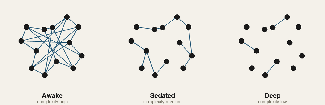
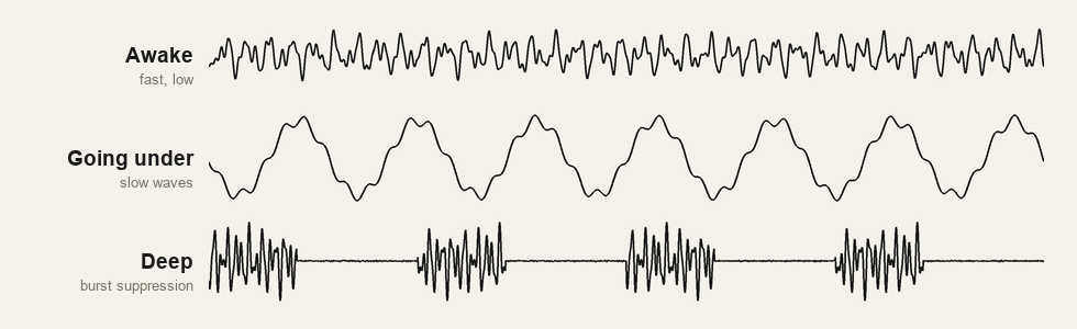
Anesthesia does not switch the brain off, it breaks the cross-talk that binds the cortex into one experience. Watch the same network come apart as it deepens, and the brain waves flatten into burst suppression. Pairs with the article Where you go under anesthesia.
1 · The network comes apart
Awake, the cortex is one densely connected whole, with information flowing between regions. As the anesthetic deepens the links thin out, and at a surgical plane the regions sit as near-isolated islands. The neurons are still alive and firing. What is gone is the conversation between them, and that is where the measure called perturbational complexity drops as consciousness fades.
2 · The brain waves flatten
On the monitor, going under walks the EEG down a staircase. Fast low activity when awake, big slow waves as you lose consciousness, and at deep levels burst suppression, where a second of activity alternates with a second of near-total silence. Push further and it flattens completely.
How this was measured, and why it does not mean we understand consciousness, is in the article Where you go under anesthesia.
TMS-EEG cortical connectivity · perturbational complexity index · the EEG stages of anesthesia.
EEG rhythms
Brain waves and sleep
A brain wave is never one rhythm. It is many stacked together. Slide the five EEG bands and watch the trace change character, then walk a whole night and see the same bands rearrange from deep sleep to dreaming.
3.5 second window
Reads likerelaxed and awake, often with eyes closedLoudest bandAlpha
Delta0.5 to 4 Hz
0%
Theta4 to 8 Hz
0%
Alpha8 to 12 Hz
0%
Beta12 to 30 Hz
0%
Gamma30 Hz and up
0%
6uV
8uV
34uV
14uV
5uV
StageAwakeInto the night0 h 00 mSleep spindles firing
What this leaves out. Real EEG is noisy and shifts across the scalp, stages blend into each other instead of switching cleanly, and the microvolt numbers here are a rough guide rather than a calibrated measurement.
Frequency bands and sleep-stage signatures follow standard EEG references, including Berger's 1929 report of the alpha rhythm and the AASM Manual for the Scoring of Sleep and Associated Events. This is an idealized synthetic model, not a real recording. Nothing here is saved and nothing is graded.
Coupled oscillators
Synchrony and binding
Twenty-four units, each blinking at its own slightly different pace, so at first the ring is a mess. Raise the coupling and let them feel each other, and they slide into one shared beat. Neuroscientists think a pull like this is how far-apart cells lock together into the rhythms tied to attention and to binding the parts of a scene into one thing.
Coupling is low. The units drift at their own paces and the synchrony reading sits near 0.
Coupling0.16
What this leaves out. This is the Kuramoto model, the simplest honest way to show phases pulling into step. Real neurons are not smooth oscillators, they couple through messy delayed synapses, and whether this kind of synchrony truly does the work of binding a scene together is still argued over. The synchrony reading is the model's own order parameter, not anything measured from a brain.
Model after Kuramoto, Y. (1975). Self-entrainment of a population of coupled non-linear oscillators. International Symposium on Mathematical Problems in Theoretical Physics. Framing follows work on gamma-band neural synchrony and the binding problem (for example Singer and Gray, 1995).
Memory and decision
Evidence to a bound
A decision, accumulating
A field of dots drifts left or right and you call the direction. The bar next to it is a model that adds up the same noisy motion until it reaches a threshold, and where you set that threshold is what trades speed against mistakes.
The motion20%
The evidencerunning
Your call, before the bar commits
or the left and right arrow keys
Watching the dots.
from the formula
from the runs
Error rate
12%
—
Decision time
0.84 s
—
Your calls will show up here once you start answering.
Speed against accuracy
Raise the threshold and the model waits for more evidence. It makes fewer mistakes but takes longer, so the marker slides down and to the right. That whole trade is drawn straight from the model's own equations.
20%
1.00
This bar is a drift-diffusion model, not a recording from a brain. A real perceptual decision builds up over hundreds of milliseconds across many neurons in areas like MT and LIP. The dots show you the motion strength, but the bar is driven by that same strength and direction rather than by these exact dots. Your own calls are one short run, not a measured study.
Model and task after Gold, J. I., and Shadlen, M. N. (2007). The neural basis of decision making. Annual Review of Neuroscience, 30, 535 to 574. Closed forms for error rate and decision time after Palmer, Huk, and Shadlen (2005) and Bogacz et al. (2006).
Reconstructive memory
The false memory
Read a short list of themed words, then take a quick memory test. One test word fits the theme perfectly but was never shown, and most people are sure they saw it.
This experiment needs a moment of interaction. Here is what it does, in case the script has not loaded.
You study a list of words that all point at one idea, sleep, without the word ever appearing. The studied words are below.
Then a recognition test asks which words you saw. The word sleep is on that test but was never in the list, and most people are certain they saw it. Memory rebuilds the gist rather than replaying a recording, so a word that fits the theme can feel just as real as the ones you read.
Roediger, H. L., and McDermott, K. B. (1995). Creating false memories, remembering words not presented in lists. Journal of Experimental Psychology, Learning, Memory, and Cognition, 21(4), 803 to 814. doi.org/10.1037/0278-7393.21.4.803
Associative memory
Pattern completion
Store a small pattern in a Hopfield network, then scribble over it. Every cell keeps
checking its neighbors and flips to match the crowd, so the grid slides step by step
back to the closest memory it holds.
Click or drag to draw. Arrow keys move the cursor and space toggles.
cell oncell offjust flipped
patterns stored
1
match to a memory
100%
energy
0.0
flips so far
0
Energy as it settles · lower is a cleaner memory
Draw
Run
This is a model, not a brain. Real neurons are not two-state switches and the brain
keeps no single energy number like this. A grid this size holds only about twenty
patterns cleanly. Store more than that and the memories blur, and a cue can settle
into a blended state that was never drawn.
Hopfield, J. J. (1982). Neural networks and physical systems with emergent collective
computational abilities. Proceedings of the National Academy of Sciences 79 (8),
2554-2558. doi 10.1073/pnas.79.8.2554
Maps and methods
Weight drugs · the real target
The appetite switch
Everyone says the weight drugs work on your stomach. Trace the real signal, and tap any part of the circuit to see what it does.
The circuit
Where these drugs actually work
Pick a source above to send a signal through the circuit, or tap any node to see what it does. The whole path runs from your gut to your brain, and never through your stomach's size or your metabolism.
Tap a node →
Hunger drive · AgRPhigh
Fullness · POMC / MC4Rlow
Food noise · rewardloud
Stomach emptyingfast
Nausea risk · area postremanone
No extra GLP-1 in the system. The hunger neurons run loud, the reward circuit flags food as urgent, and the stomach empties fast. The drive to eat stays high.
A schematic of a circuit neuroscientists are still mapping, simplified to show route and direction rather than exact wiring. GLP-1 also acts on the gut and pancreas, and the reduced eating, not any boost to metabolism, is what drives the weight loss. Built by The Neuroscience Review.
The brain GPS
Place cells and grid cells
Drag the animal around the box, or focus it and walk it with the arrow keys. Switch between two real cell types. One fires only when the animal crosses a single spot. The other fires in a repeating hexagon of spots that tiles the whole floor. Every amber dot is one spike, dropped where the animal stood, so the firing map draws itself as you move.
Place cell firing rate at the animal
0 Hz
spikes on the map 0
This is a standard model of the firing, not raw recordings. Real fields are noisier, they can drift between sessions, and a real grid is never perfectly regular. The box is one meter across, the place field is about 15 centimeters wide, and the grid spacing is about 30 centimeters.
O’Keefe and Dostrovsky (1971) found place cells in the hippocampus. Hafting, Fyhn, Molden, Moser and Moser (2005), Nature 436, 801, found grid cells in the entorhinal cortex. Firing here comes from a three cosine grid model and a Gaussian place field.
Reward prediction error
Dopamine and prediction error
Deliver a reward after the cue light a few times, then withhold it once. The modeled dopamine signal bursts at whatever it did not see coming, moves back onto the cue as the cue learns to predict the reward, and dips below baseline when a promised reward never arrives.
modeled dopamine · arbitrary units, relative to baselineModel
time within one trial, left to right · cue light then reward
Trial 1reward delivered
dopamine at the cue light
+0.00
dopamine at reward time
+1.00
The reward was a surprise, so the signal bursts when it arrives. Deliver it a few more times and watch the burst move onto the cue.
This is a temporal-difference learning model in arbitrary units. It is not a recording and it is not your dopamine. It shows the sign and timing of the reward prediction error the way Schultz and colleagues modeled it, not real firing rates, and the recordings come from dopamine neurons in the monkey midbrain. The slow backward creep of the burst from the reward to the cue is a quirk of this particular model, cleaner in the math than in the animal.
Schultz, W., Dayan, P., & Montague, P. R. (1997). A neural substrate of prediction and reward. Science, 275(5306), 1593-1599. doi.org/10.1126/science.275.5306.1593. Modeled here with temporal-difference learning.
The BOLD signal
What fMRI measures
Click to fire a neural spike. The spike is instant, but the thing fMRI actually reads, the blood-oxygen response, oozes up to its peak about 5 seconds later and slowly falls. Then move the noise and threshold sliders and watch the same blob light up or vanish.
neural spike (instant) measured signal true response threshold
Time runs left to right. The right edge is now, and the window holds about 24 seconds.
Seconds since spikeno spike yet
Signal now0.00
Threshold0.35
Blob on the mapno blob
0.15
0.35
This is the standard double-gamma model of the response, not real scanner data. Real fMRI measures blood oxygenation, an indirect stand-in for neural activity that trails it by seconds, and real activation maps come from statistics run across the whole scan, not one raw cutoff on a single voxel.
Response model from Glover, G. H. (1999), Deconvolution of impulse response in event-related BOLD fMRI, NeuroImage 9(4), 416-429. Indirect neural basis from Logothetis, N. K. et al. (2001), Neurophysiological investigation of the basis of the fMRI signal, Nature 412, 150-157.
The paper, made operable
Buy back the years
The study sorted people by how many of three midlife risks they carried. Flip them on and off and watch the dementia-free years move across the four figures it reported. These are group averages across thousands of people, not a prediction about any one person.
0years given up, a clean midlife
Group average 30.1 dementia-free years, ages 55 to 95
age 557595
How the active risks hit the small vessels
Who carries the gap. Among people with all three, the study reported 18.1 dementia-free years for women and 16.6 for men, and 19.6 for white participants and 16.0 for Black participants. The people with the most vascular risk and the least sustained treatment stand to regain the most.
What this leaves out. These are group averages, not a personal forecast. Each risk was measured once in midlife, so it is a snapshot, not a lifetime. Dementia-free years also fold in earlier death, since the same vascular damage drives heart attacks and strokes, so part of the gap is lost years of life, not only lost memory. The link is observational for all three, and only for blood pressure has a trial, SPRINT MIND, shown that treatment actually protects thinking. And a yes-or-no count of three risks is blunt, so it groups every two-of-three together, whichever two they are.
Figures from Hu, Coresh, et al., “Midlife Vascular Risk Burden and Dementia-Free Survival Years,” Neurology Open Access 2026.
A barn owl strikes in the dark by ear. Drag the mouse around and watch two tiny differences do the work. The sound reaches the near ear a hair sooner, which fixes the left to right angle, and its lopsided ears make it a touch louder above or below, which fixes the height. Together they light up one spot on a built-in map of space. Then put prism goggles on the owl and watch that map slowly slide to a new home.
Interaural time difference
0 µs
Interaural level difference
0 dB
Drag the mouse. Straight ahead the two ears hear it at the same time and the same loudness, so the map points dead center.
Days adapting0 days
What this leaves out. This is a schematic, not a recording. A real owl reads timing down to microseconds in a dedicated brainstem circuit, its map lives in the midbrain, and the numbers here are illustrative rather than measured from a bird. The prism result is real though. Eric Knudsen showed a young owl's map can slide almost all the way over to match a displaced visual world, and drift back when the prisms come off.
After Knudsen, E. I. work on the barn owl auditory space map and its plasticity, for example Knudsen (2002), Instructed learning in the auditory localization pathway of the barn owl, Nature 417, 322-328.
Next on the bench
The bench is full, and still filling.
Every experiment here runs on your own brain, right in the page, and there are more than twenty of them now. One for almost every idea the writing has reached, from a neuron finding threshold to a false memory taking hold. Each new piece still brings its own instrument, so subscribe and the next one arrives with the essay it was built for.
Subscribe →One email when a new experiment goes live.
Nothing here is saved and nothing is graded. Every result is your own single run, n = 1, not a diagnostic.
We store your theme in your browser and use only cookieless, privacy-friendly analytics, with no ads and no tracking cookies. See our privacy notice for the details.